I've been meaning to create a simple example that demonstrates how a likelihood ratio can be calculated. A few days ago, I did. The inspiration was a plot that appeared in many recent publications, which compared the various observational channels at the LHC against the standard model prediction vs. a "null hypothesis", which was the standard model without the Higgs boson. The two hypothesis were represented by two values, 0 and 1, and the various channels were marked on the vertical axis, their values plotted with horizontal error bars.
So for this example, I started with ten random data points and associated error bars, shown below.
|
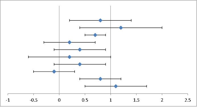 |
The null hypothesis is that the values are centered on the vertical axis at 0. The alternative hypothesis is that the values are centered on 1.
The average of these values is 0.57. Their error bars are large. The (normalized) $\chi^2$ values per degrees of freedom associated with the two hypotheses do not suggest a significant difference:
\begin{align}
\chi^2_0&=\frac{1}{n-1}\sum\limits_{i=1}^n\frac{a_i^2}{\sigma_i^2}=2.80,\\
\chi^2_1&=\frac{1}{n-1}\sum\limits_{i=1}^n\frac{(a_i-1)^2}{\sigma_i^2}=1.86.
\end{align}
However, when we compute the likelihood ratio, the picture changes. The likelihoods are calculated as
\begin{align}
L_0&=\prod\limits_{i=1}^n{\cal L}(a_i,\sigma_i)=3.73\times 10^{-7},\\
L_1&=\prod\limits_{i=1}^n{\cal L}(a_i-1,\sigma_i)=2.61\times 10^{-5},
\end{align}
where ${\cal L}(x,\sigma)$ is the Gaussian distribution of $x$ with standard deviation $\sigma$.
The ratio of $L_1$ and $L_0$ is 70.1; i.e., the '1' hypothesis is more than 70 times as likely as the '0' hypothesis.
Another way of expressing this is that if the only two competing hypotheses are the '0' and '1' cases described here, then we can normalize the likelihoods and express them as probabilities:
\begin{align}
{\cal P}_0&=\frac{{\cal L}_0}{{\cal L}_0+{\cal L}_1}=1.4\%,\\
{\cal P}_1&=\frac{{\cal L}_1}{{\cal L}_0+{\cal L}_1}=98.6\%,
\end{align}
which actually looks like a nearly $2.5\sigma$ significance.
We can also interpret this result as a prediction that as more data are collected in an experiment that yielded these results, under the assumption that either the '0' or the '1' hypothesis must be true, the data will converge on the '1' hypothesis with a probability of 98.6%.
I guess this demonstrates the statement that I found on Wikipedia, which says that ``use of the likelihood ratio test can be justified by the Neyman–Pearson lemma, which demonstrates that such a test has the highest power among all competitors''.